Information Theory for Machine Learning

Information Theory, according to Wikipedia, delves into the quantification, storage, and communication of information. In this write-up, we try to systematically understand each of underlying concept of information theory. Let’s begin by asking what “information” truly signifies.

Surprise and self-information

One way to understand information is through the concept of surprise. If an event $x$ has probability $p(x)$, how surprised should we be when it happens? Rare events should surprise us more, and a sure event ($p=1$) should not surprise us at all. The most obvious quantity with that shape is the inverse probability:

Plotting it against probability gives the curve below:

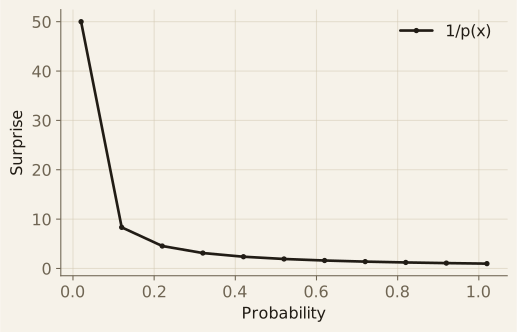
As the curve shows, this formulation gives a high information score to events with low probability, but it has two ugly properties for an honest measure of information:

• A certain event still carries one unit of surprise. $1/p(x) = 1$ when $p(x)=1$, not zero. We want the surprise of a guaranteed outcome to be exactly zero, since seeing something we already knew tells us nothing new.
• Independent events should add, but $1/p$ multiplies. If $x$ and $y$ are independent, $p(x,y)=p(x)p(y)$, so $\frac{1}{p(x,y)} = \frac{1}{p(x)}\cdot\frac{1}{p(y)}$. Learning two unrelated facts should be twice as informative as learning one, a sum rather than a product.

The function that fixes both problems at once is the logarithm. Taking $\log\!\big(1/p(x)\big) = -\log p(x)$ gives us:

The figure below plots this new score and contrasts it with the earlier $1/p(x)$:

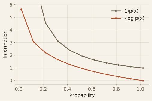
Now $I(x)=0$ when $p(x)=1$ (first problem solved), and for independent events $I(x,y) = -\log p(x)p(y) = I(x)+I(y)$ (second problem solved). Choosing $\log_2$ measures information in bits, while choosing $\ln$ measures it in nats. The base only scales the whole thing uniformly, so it changes no optimization problem. In deep-learning, we default to $\ln$ because it is the derivative-friendly choice.

Note: Shannon showed that $-\log p$ is not just one function with these properties but the only one, up to a multiplicative constant: any measure that is continuous in $p$, monotonically decreasing, and additive across independent events is forced to be $-c\log p$.

Entropy

Self-information scores a single outcome. To characterize a whole random variable rather than one event, we average self-information over the distribution itself, and that average is the entropy:

It answers a natural question: on average, how uncertain am I about $X$? Two extremes pin down the intuition:

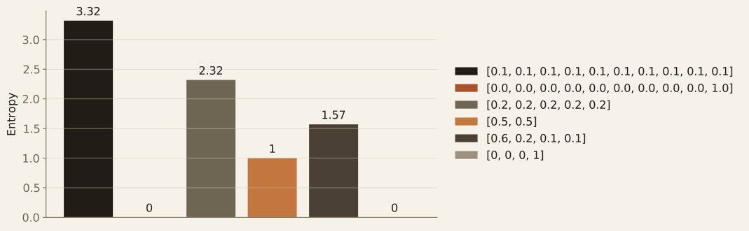
• Deterministic. If $X$ takes one value with probability 1, then $H(X) = -1\cdot\log 1 = 0$. There is nothing to learn from a sample, because we already know the answer.
• Uniform. If $p(x)=1/K$ for each of $K$ outcomes, then $H(X) = -\sum \frac{1}{K}\log\frac{1}{K} = \log K$, the maximum possible for a $K$-outcome distribution. Every outcome is equally surprising.

The figure below makes this concrete, showing the entropy of several distributions: largest for the uniform ones and zero for the deterministic ones.

In ML, entropy shows up wherever we want a distribution to be “spread out”: exploration bonuses in RL, regularizing softmax outputs to avoid overconfidence, and encouraging diverse generations in language models via temperature.

Joint and conditional entropy

Entropy describes the uncertainty in one variable. As soon as we have two variables with joint distribution $p(x,y)$, the same averaging idea produces two more quantities.

Joint entropy is the uncertainty in the pair $(X,Y)$ taken together:

Conditional entropy is the uncertainty left in $Y$ after we have already seen $X$:

If $X$ already determines $Y$, this is zero; if $X$ tells us nothing about $Y$, it collapses back to $H(Y)$.

Chain rule. These two quantities combine cleanly:

In words, the uncertainty about the pair equals the uncertainty in the first variable plus the leftover uncertainty in the second once the first is known. The proof simply factors $p(x,y)=p(x)\,p(y\mid x)$ inside the logarithm and splits the sum, the same move (turning a product of probabilities into a sum of log-probabilities) that powered the definition of self-information. It extends to any number of variables in the obvious way.

Cross entropy

Every quantity so far has used a single distribution, measuring a variable against its own probabilities. Real machine learning almost always involves two distributions on the same outcomes: a true distribution $p$ (the data, the labels, the world) and a model $q$ we are trying to fit. The first quantity that relates them is the cross-entropy of $p$ relative to $q$, the average surprise that the model $q$ assigns to samples drawn from the true distribution $p$:

The surprise of observing $x$ under the model is $-\log q(x)$, which is large when $q$ thinks $x$ is rare. The world, however, sends samples from $p$ rather than $q$, so the relevant average is taken under the true distribution. Intuitively, $H(p,q)$ is the per-sample description cost of building our encoding around $q$ and then running it on samples from $p$: we pay more nats per symbol than we would have under the right model.

The figure below shows cross-entropy for a few source and target pairs, spiking when the model places little probability on outcomes the truth considers likely:

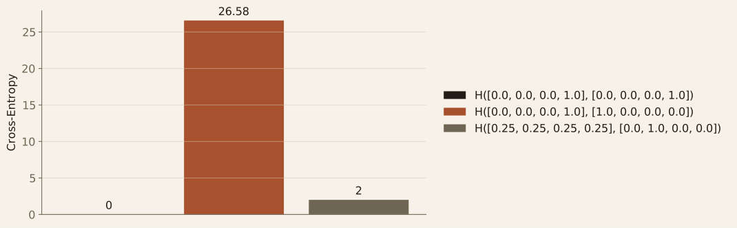
It helps to check that the cross-entropy definition behaves the way we would expect, and two observations do exactly that. First, when $q=p$, cross-entropy collapses back to plain entropy, $H(p,p)=H(p)$, so the right model wastes nothing. Second, $H(p,q)\neq H(q,p)$ in general, because the first argument is the sampling distribution (which outcomes we actually see) while the second is the scoring distribution (how surprised the model is). Swap them and both roles flip. That asymmetry reappears, sharper, in the quantity we turn to next.

KL divergence

Cross-entropy measures the total cost of describing $p$‘s samples with $q$. Some of that cost is unavoidable, since even the perfect model still pays $H(p)$. Subtracting this floor leaves the extra cost of using the wrong model, and that excess is the Kullback–Leibler divergence:

Read it as a question: on average over samples from $p$, how many extra nats does it cost to describe them using $q$ instead of $p$? If $q=p$, every $\log(p/q)$ term is $\log 1 = 0$, so $\mathrm{KL}(p\parallel p)=0$. The further $q$ drifts from $p$, the higher the penalty.

A Jensen-inequality argument on the concave logarithm shows that $\mathrm{KL}(p\parallel q)\ge 0$ always, with equality only when $p=q$ almost everywhere. This non-negativity is not an extra axiom; it is exactly the statement that we cannot out-compress the source by using the wrong model. A few properties are worth internalizing:

• Non-negative: $\mathrm{KL}(p\parallel q)\ge 0$, and zero only when $p=q$.
• Asymmetric: $\mathrm{KL}(p\parallel q)\neq \mathrm{KL}(q\parallel p)$ in general, so it is not a distance.
• Mode behavior matters. $\mathrm{KL}(p\parallel q)$ punishes $q$ for putting low mass where $p$ has mass (mass-covering, so $q$ spreads out), while $\mathrm{KL}(q\parallel p)$ punishes $q$ for putting mass where $p$ has none (mode-seeking, so $q$ collapses onto a peak).
• Which direction shows up where. Variational inference (including VAEs) and most policy-gradient RL use the reverse form $\mathrm{KL}(q\parallel p)$, because that is the side we can sample from, since the expectation is taken under $q$, the distribution we control. Maximum-likelihood training uses the forward form $\mathrm{KL}(p\parallel q)$, because data gives us samples from $p$ for free. Availability of samples, not aesthetics, picks the direction, and the direction picks the qualitative answer.

Cross entropy and KL: the relation

We arrived at KL by subtracting $H(p)$ from cross-entropy, so rearranging recovers the relation directly:

The first term is the irreducible uncertainty in $p$, fixed by the source, and the second is the gap our model leaves on the table. Cross-entropy is the absolute description cost, while KL is the part of that cost that is our fault.

This identity drives most of supervised deep learning: minimizing $H(p,q)$ over $q$ is the same as minimizing $\mathrm{KL}(p\parallel q)$, because $H(p)$ does not depend on the model. The two objectives differ only by an additive constant that the gradient never sees.

In supervised classification, $p$ is the one-hot label distribution ($p(y^\star)=1$ and zero elsewhere) and $q$ is the model’s softmax $q_\theta(y\mid x)$. Since the one-hot $p$ has $H(p)=0$, cross-entropy and KL coincide exactly, and both reduce to a single term:

which is the negative log-likelihood of the true label. So “training a classifier with cross-entropy loss,” “minimizing KL to the one-hot label,” and “maximum likelihood estimation” are the same procedure described in three vocabularies.

Beyond unifying these three views, cross-entropy has a practical virtue that explains why it became the default loss: it is remarkably well-behaved under gradient descent. If $q_\theta$ is a softmax over logits $z\in\mathbb{R}^K$, a short computation gives

The gradient with respect to the logits is simply prediction minus target. There is no softmax derivative to chase and no vanishing-gradient pathology even when $q_\theta$ is confidently wrong. Every other natural classification loss, such as squared error on probabilities or hinge, gives up some of this, because the logarithm is exactly what undoes the exponential in the softmax. This identity is why cross-entropy is the default and why training stays numerically stable across many orders of magnitude in $q_\theta$.

Label smoothing. Replace the one-hot target with a softer one that gives the true class $1-\epsilon$ and spreads $\epsilon$ over the rest. The target $p$ now has nonzero mass on every class, so $q$ can never push a logit to $-\infty$ without paying for it. This gently prevents the model from becoming arbitrarily confident, which often improves calibration and generalization. More broadly, almost every “match this distribution to that one” loss in deep learning is a KL in disguise, and most of those KLs reach us through the cross-entropy door.

Jensen–Shannon divergence

KL answers an inherently asymmetric question: how badly does $q$ describe samples from $p$? The moment we try to use it as a general-purpose distance between two distributions on equal footing, three pathologies surface. It is asymmetric, it is unbounded (taking values in $[0,+\infty]$), and it blows up to $+\infty$ whenever the two distributions have disjoint support. That last case is common, since two distributions on low-dimensional manifolds in a high-dimensional space generically have disjoint support, so KL reports “infinitely far apart” and offers no usable gradient.

The Jensen–Shannon divergence fixes all three problems by measuring each distribution’s gap to their average rather than to each other. With $m=\tfrac12(p+q)$:

Because $m$ inherits the union of the two supports, neither KL inside can blow up. JSD is symmetric, bounded in $[0,\log 2]$ (the upper limit reached exactly when $p$ and $q$ have disjoint support), and $\sqrt{\mathrm{JSD}}$ is a genuine metric. Collecting terms gives a clean identity in entropy alone:

So JSD is the entropy of the mixture minus the mixture of entropies, which is the Jensen gap of entropy under mixing and the source of its name.

Where it shows up: GANs. For the optimal discriminator, the original GAN objective reduces to $\min_G 2\,\mathrm{JSD}(p_\text{data}\parallel p_g) - 2\log 2$. But the very property that makes JSD well-defined on disjoint supports, namely saturating at $\log 2$, is also what kills its gradient in practice. When $p_\text{data}$ and $p_g$ live on different manifolds, JSD equals $\log 2$ almost everywhere and the gradient vanishes. This is the pathology that Wasserstein GANs were designed to escape, by switching to a divergence whose value tracks geometric distance rather than support overlap.

Mutual information

JSD compares two arbitrary distributions. One particular comparison is so useful that it earns its own name: measuring a joint distribution against the product of its marginals. That is mutual information, and it asks how much does knowing $X$ reduce my uncertainty about $Y$? Equivalently, it asks how far the joint $p(x,y)$ sits from the product $p(x)p(y)$ that would hold if the two variables were independent:

Three equivalent rewrites are worth knowing by heart, since each gives a different angle on the same number:

Mutual information is symmetric, non-negative, and zero exactly when $X$ and $Y$ are independent. Unlike correlation, it captures any statistical dependence rather than only linear ones. In representation learning it is the quantity we try to maximize between an input and its embedding (to preserve information) and minimize between an embedding and a nuisance variable (to remove it).

Information gain: MI under another name. The quantity $H(Y)-H(Y\mid X)=I(X;Y)$ is called information gain in two ML lineages. In decision trees (ID3, C4.5) it scores a feature split, where we pick the $X$ that maximizes $I(Y;X)$. In Bayesian active learning and RL exploration it scores a query or action by how much its outcome would shrink the posterior over parameters. Different names, same mutual information.

Two structural results: DPI and Fano

Mutual information obeys two inequalities that appear often enough in ML to deserve their own names.

Data processing inequality. If $X\to Y\to Z$ forms a Markov chain (so $Z$ depends on $X$ only through $Y$), then

Post-processing cannot create information. A learned representation $Y$ of an input $X$, followed by any classifier $Z=f(Y)$, can at best preserve information about $X$ and never manufacture more. This is the formal reason that every layer of a deep network is at best information-preserving in $X$, and that lossy compression has a real floor.

Fano’s inequality. Where DPI says high mutual information is necessary for good prediction, Fano makes the statement quantitative. The conditional uncertainty $H(Y\mid X) = H(Y)-I(X;Y)$ lower-bounds how well any prediction rule can do. If $X$ and $Y$ are not informative enough about each other, no classifier, however clever, can drive the error below the Fano floor. This is the inequality behind information-theoretic lower bounds on sample complexity.

KL in variational inference: the ELBO and VAEs

These quantities are not only descriptive; they appear directly inside training objectives. The clearest example is the variational autoencoder, a latent-variable generative model with three pieces: a prior $p(z)$ over latents (usually a standard Gaussian), a decoder $p_\theta(x\mid z)$ that maps a latent back to a distribution over observations, and an encoder $q_\phi(z\mid x)$ that maps an observation to a distribution over latents. The encoder produces Gaussian parameters $\mu$ and $\sigma$, and the reparameterized sample $z=\mu+\sigma\odot\epsilon$ with $\epsilon\sim\mathcal{N}(0,I)$ is passed through the decoder to a reconstruction.

The goal is the same as for any generative model: maximize the log-likelihood $\log p_\theta(x) = \log\int p_\theta(x\mid z)p(z)\,dz$. The trouble is that this marginal is intractable. The integral has no closed form once $p_\theta$ is a neural network, and naive Monte Carlo from the prior collapses, because the prior covers the latent space democratically while the integrand cares about a tiny neighborhood, and democratic sampling does not mix well with concentrated mass.

The variational move introduces a tractable surrogate posterior $q_\phi(z\mid x)$ and applies Jensen’s inequality to the logarithm:

The gap between this evidence lower bound and the true log-likelihood is exactly $\mathrm{KL}(q_\phi(z\mid x)\parallel p_\theta(z\mid x))$, so tightening the bound is pushing the approximate posterior toward the true one. The two ELBO terms have clear physical meanings. Reconstruction asks the decoder to actually rebuild $x$ from its latent, and the KL term keeps the encoder honest by stopping it from inventing latent codes that look nothing like samples from the prior. The whole VAE objective is one entropy quantity balanced against one KL.

The information bottleneck

The VAE balances reconstruction against a KL penalty. A closely related idea makes the trade-off between compression and prediction completely explicit. A representation $Z$ of an input $X$ used to predict a target $Y$ should forget everything about $X$ that is not useful for $Y$, and the information bottleneck formalizes this as a trade-off:

The first term penalizes how much $Z$ remembers about $X$ (compression), and the second rewards how much $Z$ tells us about $Y$ (prediction). The coefficient $\beta$ slides between a maximally compressive and a maximally predictive representation. The deep variational information bottleneck replaces the intractable mutual informations with variational bounds and trains end to end, and algorithmically it looks much like a supervised VAE: the same KL-versus-reconstruction trade-off with a different motivation.

Estimating mutual information with neural networks

Both the VAE and the information bottleneck lean on mutual information, which is easy to write down and notoriously hard to estimate. In high dimensions we cannot enumerate $p(x,y)$, and density-ratio estimation is fragile. Two ideas have become standard.

MINE uses a Donsker–Varadhan bound on KL. It trains a network $T_\theta(x,y)$ to distinguish samples from the joint $p(x,y)$ from samples drawn from the product of marginals $p(x)p(y)$, and reads off a lower bound on $I(X;Y)$ from how well the network does. The network itself is a learned critic.

InfoNCE (contrastive predictive coding) optimizes a lower bound on mutual information with a noise-contrastive softmax. Given a query $x$, one positive $y$ drawn from the joint, and $K-1$ negatives drawn from the marginal, the model classifies which candidate is the positive. The resulting loss is the backbone of essentially all modern self-supervised learning (SimCLR, MoCo, CLIP). The maximum mutual information any InfoNCE-style estimator can certify is $\log K$, a fundamental ceiling, which is why batch size matters so much in contrastive learning.

Entropy as a regularizer: maximum-entropy RL

Mutual information served as a training signal in the last few sections. Entropy can play the same role directly. A pure reward-maximizing objective in reinforcement learning collapses the policy onto whichever action looks best so far, which kills exploration. Maximum-entropy RL adds an entropy bonus to the reward, so the agent chases return while keeping its action distribution spread out:

The temperature $\alpha$ trades exploitation against exploration, and Soft Actor-Critic is the canonical implementation.

The entropy term is not a standalone trick; it is a KL in disguise. For a uniform reference policy $\pi_0(a\mid s)=1/|\mathcal{A}|$,

so maximizing entropy is, up to a constant, the same as minimizing the KL from the policy to a uniform prior. Replace the uniform $\pi_0$ with a learned reference and we recover the KL-to-reference objective used in RLHF and in PPO-with-reference. The entropy bonus, the KL penalty in RLHF, and the trust-region term in PPO are all the same regularizer with different reference distributions.

From discrete to continuous

Every formula so far has used sums over a discrete alphabet. Moving to continuous variables means replacing sums with integrals and probabilities with densities, which turns entropy into differential entropy:

The change from $H$ to $h$ flags that something is different. Differential entropy can be negative, because a density can exceed 1 on small regions, so $-\log p$ can be negative and the integral can come out negative too. It is best treated as a relative quantity rather than an absolute one. It is also not reparametrization-invariant, since a change of variables leaks in a Jacobian term, so rescaling a VAE’s latent changes its entropy.

The reassuring news is that KL and mutual information stay well-behaved in the continuous case, because the Jacobian appears in both densities and cancels in the ratio $p/q$ or $p(x,y)/(p(x)p(y))$. This is why almost every information-theoretic objective in deep learning is a KL or a mutual information rather than a raw entropy. Entropy still appears, in the ELBO and in maximum-entropy RL, but only inside combinations where the bad behavior cancels.

Summary

Three quantities have carried this entire story of information theory. First, Entropy measures the uncertainty inside a single distribution, built up from the surprise of one outcome. Second, KL divergence measures the gap between two distributions, the excess cost of describing one with the other. Third, Mutual information measures how tightly two variables are coupled, and it is itself a KL between a joint distribution and the product of its marginals.

Everything else has been a re-skin of these three concepts. Cross-entropy is entropy plus a KL. The classification loss, maximum likelihood, and KL to a one-hot label are one objective wearing three names. The VAE balances a reconstruction term against a KL to the prior, the information bottleneck trades one mutual information against another, contrastive learning maximizes a bound on mutual information, and maximum-entropy RL is a KL to a reference policy in an entropy costume. Even the move from discrete to continuous leaves KL and mutual information intact while only entropy needs extra care.